This work describes the application of neural networks in the modeling of hot rolling processes. This relatively new technique of Artificial Intelligence was conceived more than fifty years ago, but it only became really feasible with the arrival of low cost computer processing power. The first papers about its utilization in the hot rolling field were published in 1992. Although the first results were promising, there is still some lack of confidence about its real performance under industrial conditions, which is preventing the exclusive use of this new tool in the modeling of hot rolling processes. However, neural networks are already being used, as a standard feature, in hybrid automation models for hot strip mills, where they calculate adjusting coefficients for theoretical models. However, continuous use of these tools and its continuous development certainly will contribute to increase the general confidence in this revolutionary method and pave the way for a more intensive application in practical cases.
- INTRODUCTION
The advent of revolutionary steelmaking processes, new materials like high performance polymers and ceramics, and a chronic excess of capacity production made steel market very competitive. If a steelmaker wants to keep or expand its market share, it must offer products with excellent quality at an affordable price. One of the keys to achieve this goal is the automation of the steelmaking process. In fact, this is one of the major stages of evolution in a steel plant, as it improves both process and product consistency, minimizes costs and make production control easy. All these factors promote a significant increase in the process cost/benefit ratio.
The automation of hot rolling processes requires the development of several mathematical models for the simulation and quantitative description of the industrial operations involved.
The main feature of the neural networks - the establishment of complex relationships between data through a learning process, with no need to previously propose any model to correlate the desired variables - makes this technique very attractive in the modeling of processes where traditional mathematical modeling is difficult or impossible. Besides that, they are almost immune to noise or spurious data. The development of neural network models is relatively quick and, in most cases, simple. Several researchers performed off-line tests on the modeling of hot rolling processes using this technique, frequently getting good results.
However, practical applications of this technique in the field of hot rolling are very scarce, mainly due to the lack of confidence about its performance. This distrust on neural networks arises from many factors. First of all, only recently this technique became feasible, with the increasingly wide availability of low-cost computer power. Besides that, as the mathematical foundations of neural networks are not still completely developed, no one knows exactly the mechanisms of its learning, that is, it is unknown how a neural networks calculates a given result. So, frequently they are considered as potentially unreliable "black boxes". Under some aspects this is a justified attitude, as a wrong decision taken by an industrial automation system can lead to disastrous failures and high economical losses.
One additional aspect to be noted is the natural inertia to modify existing automation systems that are working well. The natural field of application for a new technique like neural networks is in hot rolling mills that do not have automation systems yet. However, in these equipments, the lack of instrumentation, data acquisition and process computers hindered the on-line use of this technique.
Neural networks can be used in several ways to model a given process. They can be used alone, but the mentioned lack of confidence on this technique has prevented this kind of approach in real world applications, at least in the case of hot rolling.
Other approach is the use of hybrid Artificial Intelligence systems, like neural networks-expert systems and neuro-fuzzy logic [1]. Few examples of this technique can be found in the field of hot rolling up to this moment.
An alternative that is being popular is the application of neural networks for the calculation of correction factors to be used in traditional mathematical models that control a given process [2]. That is, a hybrid traditional mathematical process-neural networks, where the neural network act as an assistant to the mathematical model. This kind of neural network is commonly called parameter network. For example, it can calculate heat transfer coefficients for a traditional heat flow mathematical model to be applied in the control of a slab reheating furnace.
Another example of this kind of hybridization is the so-called correction network. In this case, the traditional mathematical model calculates its best value for the process that is being controlled, while a neural network simultaneously produces the estimate of the inherent error in the mathematical model's approximation. In this case, the neural network is an equal partner to the mathematical model.
A variation of this approach is the synthesis network, a technique still in investigation [2]. In this case, mathematical models pre-process the entry data, yielding intermediate results that feed a neural network that calculates the desired target value from these highly compressed intermediate results. Additional parameters can be directly input to the neural network. An example of this approach is the pre-calculation of the strip thickness profile to be got in the finishing train of a hot strip mill. In this case, a traditional mathematical model calculates the thermal crown, wear, bending of the work rolls and the resulting roll-gap profile under load for each rolling stand. These calculated values of the resulting roll-gap profile for all rolling stands and the respective strip tensions feed a neural network that calculates the profile of the finished strip.
The advantages of the use of the combinations of mathematical models and neural networks are as follows [2]:
- SIZING SLABS FOR PLATE ROLLING
A very first trial on the application of neural networks in the field of hot rolling was developed at Usiminas, a Brazilian steelworks [3]. It was developed a neural network to replace a previous regression equation used for the calculation of the dimensions of the slab to be rolled at the plate mill, aiming minimal metal discard after hot rolling.
Some advantages are inherent to the use of neural networks instead of multiple regression equations [4]. There is no need to select the most important independent variables in the data set, as neural networks can automatically identify them. The synapses associated to irrelevant variables readily show negligible weight values; on its turn, relevant variables present significant synapse weight values. As said previously, there is also no need to propose a function as model, as required in multiple regression. The learning capability of neural networks allows them to "discover" more complex and subtle interactions between the independent variables, contributing to the development of a model with maximum precision. Besides that, neural networks are intrinsically robust, that is, they show more immunity to noise eventually present in real data; this is an important factor in the modeling of industrial processes.
Obviously, the forecasting performance of a slab sizing model will be consistent only if several operational parameters are kept under control: weight and dimensions of the slabs; precision of the pass schedules, including the broadsizing step; distribution of strain in the broadsizing step; plate crown and scale losses during the reheating of the slab. Other factors also must be considered, like the specific characteristics of the process of slab production (continuous cast or from ingots rolled at the slabbing mill), rolling type (normal or controlled) and broadsizing ratio.
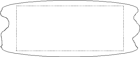
It is well known that the rolling stock produced after plate rolling does not present an exact rectangular shape, as can be seen in figure 1. The required rectangular plates are extracted from the rolling stock through the trimming of its edges. In order to maximize the metallic yield of the process, the length of the original slab must be calculated precisely, in such a way that the dimensions of the rolling stock permits the extraction of the desired plate and the lengths of the discarded portions are minimal.
Unfortunately, the paper does not give details about the former regression equation, nor the parameters used in the developed
neural network, except that it is of the back-propagation type, with two neurons in the input layer, five in one hidden layer and
one neuron in the output layer. According to the authors of this paper, the number of neurons of the hidden layer of this neural
network was calculated after the Hecht-Kolmogorov's theorem, which affirms that the optimum number of neurons of a hidden
layer is equal to twice the number of input neurons plus one [3].
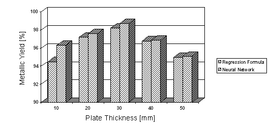
This neural network was trained with data measured from 239 rolling stocks. Figure 2 shows the improvement in the metallic yield that was got with the use of this neural network. This amelioration can be summarized by the following parameters: increase of 0,5% in the plate-slab programmed yield; increase of 1,0% in the trimming yield and increase of 0,32% in the inspection yield.
- MODELING THERMAL PROFILE OF SLABS IN THE REHEATING FURNACE
At Cosipa, another Brazilian steelmaker, thermal profiles of slabs being reheated are periodically collected at the plate mill line. These profiles are measured with an instrumented slab, which has drilled holes at several locations and depths. Chromel-alumel thermocouples are inserted into these holes and connected to a data logger, which collects all the temperature evolution of these points during slab reheating. The data logger is sheltered in a stainless steel box coated with rock wool and filled with water and ice.
It was decided to develop a neural network model to forecast the inner temperature of the slabs being reheated as a function of their reheating time and their superficial temperature [5]. This is a case with a relatively easy mathematical solution, and thus adequate to allow a comparison between the performance of the neural network and the conventional numerical models.
With this purpose in mind, a neural network with three layers was developed, after several configuration trials:
Data was got from an instrumented slab with the following dimensions: 157 mm (thickness), 1025 mm (width) and 5600 mm (length). It was reheated in a pusher furnace. More information about data used in this work can be found elsewhere [6].
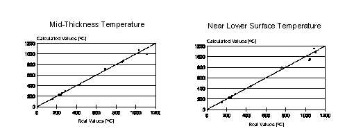
It was verified that this neural network showed its best performance forecasting the mid-thickness temperature of the slab, with Pearson's correlation coefficient r about 0.997 and standard error of estimate of 26.5oC. The worst performance of this neural network occurred during forecasting the temperature near the lower surface of the slab, that is, at a distance of about 6 mm from this surface: its results showed a Pearson's correlation coefficient r of approximately 0.993 and standard error of estimate of 36.6oC. Figure 3 shows the dispersion plots of the calculated and real temperatures of both two points considered.
The performance reached by this neural network was found adequate, as it was similar to previously developed mathematical
models, which showed errors of approximately 30oC.
- MODELING HOT STRENGTH OF STEEL
Hot strength can be defined as the stress that begins and keeps the yielding of a material in a uniaxial stress state. It is one of the fundamental properties of a material under high temperature. In the case of metals being rolled, the knowledge of its magnitude is vital for the correct designing of the mechanical and electrical components of the rolling stands, as well in the development of mathematical models and automation algorithms for the hot rolling process.
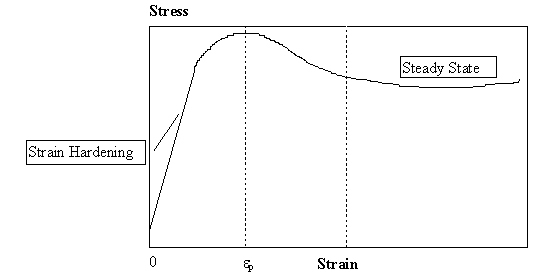
Hot rolling of steels normally occurs at temperatures corresponding to its austenitic range. Figure 4 shows schematically a typical stress versus strain curve of steel at high temperature. As can be seen from this picture, three steps characterize this curve: strain hardening, dynamic recrystallization and steady state. During the initial step of strain hardening stress grows monotonically. As soon as stress reaches its maximum value, the advent of dynamical recrystallization causes a lowering on its magnitude, down to a steady-state value, which is approximately constant or eventually shows a cyclical behavior, which denotes an "equilibrium" between strain hardening and recovery processes.
In the last 30 years several empirical equations were developed to model the hot strength of steel in function of
thermomechanical parameters like temperature, strain and strain rate. The most famous are Tarokh, Samanta, Hajduk,
Tegart, Rossard and Jäckel. Normally these equations only consider the strain hardening step of the curve stress x
strain. Few models, like Jäckel, covers all the strain range, but normally they consist of two or more equations, each one
describing a step of the curve. Its application is not always easy, as real hot strength curves are not always well-behaved as the
didactical example of figure 4. This fact makes difficult to identify the corresponding strain ranges to be applied to the several
equations that constitutes the full range model. Some other models include the effect of the chemical composition of steel (Shida,
Misaka). The Shida model also considers the softening that occurs in steel near the Ar3 temperature.
Other possibility for modeling hot strength of steels is the application of interpolation methods using large multidimensional data bases. However, memory requirements for this kind of approach are huge, making it practically unfeasible, at least up to this moment.
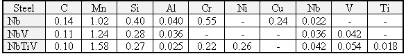
A first tentative of comparison between conventional empirical equations for the calculation of hot strength of steels and neural networks used data available from hot torsion tests of HSLA steels. The samples were heated at 1150oC during 30 minutes. After that, the temperature of the specimen was reduced down to the aimed value. Tests were isothermically performed under temperatures of 1100, 1000, 900 and 800oC, and under strain rates of 0.1, 1 and 10 s-1. Six empirical equations were used for the calculation of hot strength from temperature, strain and strain rate in the strain hardening step of the curve hot strength versus strain: Tarokh, Samanta, Hajduk, Tegart, Rossard and the strain hardening equation of the model of Jäckel. The best fitted neural network for this purpose was of the back-propagation type, with three neurons in the input layer, seven neurons in one hidden layer and one output neuron. The number of neurons in the hidden layer was calculated according to the already mentioned Hecht-Kolmogorov theorem.
The chemical composition of the steels can be seen in table I. Data used in the non-linear regression program for the parameter fitting of the empirical equations and during the learning/testing steps of the neural network was got directly from the stress versus strain curves determined in the hot torsion machine, without any pre-processing.
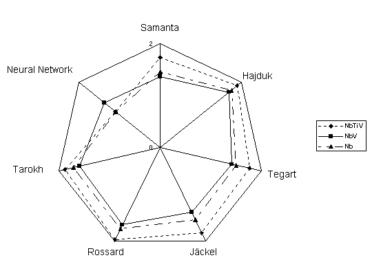
The radar-type graphic in figure 5 shows that neural networks had a clear better forecasting power than the previous empirical
equations: the best empirical model (Samanta) presented a mean standard error of estimate of approximately
1.5 kgf/mm2, whereas the neural networks showed a value of 1.2 kgf/mm2. This value was
calculated during the testing step of the neural network, after its full training, using a data set not used during its training.
Besides that, it was possible to train these neural networks with data from the full strain range of the curve hot strength versus
strain. That is, one single neural network can model the strain hardening, dynamic recrystallization and steady state steps of this
curve. The neural networks used in this case have the same topology as the previously described. Its standard error of estimate
of calculated during the testing after the training step was approximately 1.7 kgf/mm2. This kind of modeling can
not be performed with the conventional empirical equations cited here. Besides that, the use of neural networks does not require
the division of the hot strength curve in distinct steps, a kind of task which is frequently hard. This made the modeling of the full
hot strength versus strain curves very easy and quick. The best agreement given by the neural network for the dynamic
recrystallization region was also verified in other works [8] for an austenitic stainless steel.
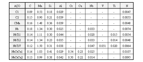
This work was later expanded to a more wide selection of carbon and HSLA steels [9]. The chemical composition of these steels can be seen in table II. The specimens were heated to 1100oC for 15 minutes, and then cooled down to the aimed temperature. Tests were isothermically performed under temperatures of 1100, 1000, 900 and 800oC, and under strain rates of 0.5, 1 and 5 s-1. The same six empirical equations cited before were used for the modeling of hot strength from temperature, strain and strain rate in the strain hardening step of the curve hot strength versus strain. The neural network used in this work was slightly different from the previous work: it has seven neurons distributed in two hidden layers (four in the second layer and three in the third layer). This arrangement showed to be better than the previously used. Data used in the non-linear regression program for the parameter fitting of the empirical equations and during the learning/testing steps of the neural network was previously processed. All the hot strength versus strain curves got from the torsion tests were smoothed using a modified Fourier's transform technique and compensated for the adiabatic heating effect arising from hot deformation.
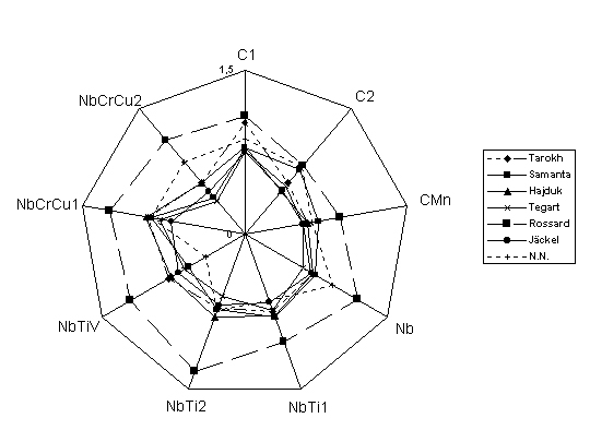
Surprisingly, in this case neural networks did not show the best forecast power, as can be seen in the radar graphic of figure 6.
Considering the performance observed in all steels, the forecast power of the empirical models of Tegart, Jäckel, Samanta and
Hajduk were greater than of the neural networks. The situation is even worse when one considers only carbon steels; in this
case, also the Samanta model surpasses the forecast power of the neural networks. However, considering HSLA steels alone,
only the equations of Tegart, Jäckel and Samanta are superior to the neural networks.
A probable reason for this unexpected conclusion can be attributed for the greater precision achieved in the models developed
in [9] in comparison with the forecast power reported in [7]. In fact, the global standard error of estimate of the best model got
in [7] has a value of approximately 1.2 kgf/mm2, while the same parameter in [9] was about the half of this value -
0.63 kgf/mm2. This better precision result from a better experimental practice and from data smoothing procedures carried out
in [9], which minimized the random errors present in the raw data. This enhanced the mathematical relationships between the
variables, which simultaneously improved the forecast power of the empirical equations and minimized a great advantage of the
neural networks, that is, its immunity to noise and spurious data. So, in the first work [7], which was based on raw data from
torsion tests, the better forecast power of neural networks certainly arosed from its inherent noise filtering effect in raw data.
This condition, however, would be no longer true in the next work [9].
Other authors also got very good results modeling hot strength of specific steels in function of the thermomechanical parameters. An example is a three layer, feed-forward neural network for the calculation of hot flow strength of an extra-low-carbon steel from temperature, strain grade and strain rate. Best results were got with a hidden layer with 14 neurons. The relative errors were within ±5%, with the exception of some few points at low strains [10].
From the good results got from these models of hot strength, it was almost unavoidable to trial neural networks to forecast hot strength not only from thermomechanical parameters, but also including the chemical composition of steel as well. After all, neural networks can identify the complex relationships between hot strength and chemical composition better than any empirical model. So, the work described in [9] was extended, including the effect of the chemical composition of steel [11]. A neural network for the prediction of hot strength from chemical composition of steels and hot forming parameters was then developed. This perceptron had 13 neurons in the input layer (strain temperature, degree and rate; carbon, manganese, silicon, aluminum, copper, chromium, niobium, titanium, vanadium and nitrogen contents). The total number of neurons in the hidden layers was 27, making an analogy with the theorem of Hecht-Kolmogorov [4]; they were uniformly distributed in three hidden layers, each one with 9 neurons.
The output layer, obviously, had only one neuron, with the predicted value of hot strength. This model revealed a very good performance: Pearson correlation coefficient r of 0.939 and a standard error of 11.8 MPa. This precision is inferior to the performance of hot strength models developed for specific alloys [9], but is very good for a model including chemical composition. This trained neural network was converted in a simple BASIC subroutine for use in mathematical models for off-line calculation of hot rolling load and pass schedule for the COSIPA plate mill.
A neural network is as good as the data used during its training step. The alloys studied in this work were selected according to its participation in the productive mix of the plate mill. Unfortunately, this criterion was not adequate from a scientific standpoint. Another problem was the scarcity of data, as only nine steels are available to develop this model that can involve up to ten chemical elements. In the example of table II, one can see that C content of the considered steels varies between 0.09 and 0.16%, while the range of Mn content is from 0.53 to 1.50%. However, C content is roughly proportional to Mn content. So, if a neural network is trained to consider the effect of chemical composition using these data, its results for a test steel containing, for instance, 0.16% C and 0.53% Mn, are potentially unreliable. These single values of C and Mn are within the range used in the training of the neural network, but data used during its training did not include this particular combination of these elements, that is, "high" C and "low" Mn. In fact, this case constitutes an extrapolation of the available data and, in this case, the predictive power of the neural networks is doubtful.
A neural network can be ideally trained to "learn" the effect of chemical composition in hot strength only if the data set available includes the results of tests performed with steels which chemical compositions cover all situations possible. This only can be made using a factorial experimental design, and certainly will involve the testing of some dozens or even hundreds of steel alloys. The work and cost involved in such research project would be very high if it would be developed from scratch. A possible solution to minimize this problem could be cooperative work between research institutions in this field, through the sharing of hot strength data.
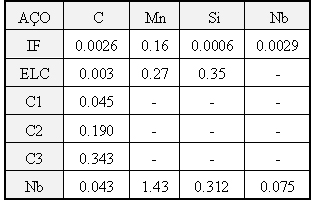
Recently some results were published [12] about the modeling of hot strength of steels from thermomechanical parameters and chemical composition. They tested six steels, which chemical composition can be seen in table III: an I.F. steel, an extra-low C steel, three low C steels and one Nb steel. Hot strength was determined using isothermal compression tests with cylindrical samples, with exception of a low C steel, which was tested using isothermal ring compression tests. These steels were tested under temperatures varying from 860 to 1100oC and strain rates from 0.001 to 1 s-1. The input data of the neural networks included temperature, strain, strain rate, C, Mn, Si and Nb contents. Trials showed that the best results were got with one hidden layer with 25 neurons. The output layer, of course, was constituted of a single neuron, the value of hot strength. Input data included the full range of the hot strength versus strain curve, that is, the steps of strain hardening, dynamic recrystallization and steady state steps.
The predictive power of the neural network was very good. After a training step with 60,000 iterations, it showed an average
error of approximately 0.10% during the test step with data not showed during the training step. The standard deviation of this
error was of 3.77%, and the maximum error was about 18%. The predictive performance of this neural network was better than
some empirical equations (Wang, Voce and Jonas) and even than a fuzzy inference model.
As tests were performed with data deriving from the same steels that generated data for the training step of the neural network, this work does not demonstrate the effective capability of the neural network to model the effect of the chemical composition on hot strength. This only could be checked if the neural network would be tested with data from a steel with different chemical composition from the steels that originated data for the training step. Once more, the problem of the scarcity of hot strength data appears. As it was available data from only six steels, the use of data from one alloy only for testing purposes certainly would impair the predictive power of the neural network, as these data would not be available for its training step.
Other work [13] deals specifically with the prediction of hot strength, taking in account the softening that occurs during rolling of extra-low C steels near the Ar3 temperature, that is, the temperature at which austenite decomposition begins during cooling. The chemical composition of the steel studied in this work is the same as the ELC alloy mentioned in table III, as well the experimental procedure for the determination of the hot strength data. The neural network developed in this paper was specific for this kind of steel. Its input layer has four neurons, corresponding to temperature, strain, strain rate and a so-called phase index. The function of this last parameter was to make the neural network distinguish the flow curves in the various regimes: austenitic, austenitic-ferritic and ferritic. This phase index is the volume fraction of transformation of austenite in ferrite. There were two hidden layers, each one with 12 neurons. Of course, the output layer was constituted of only one neuron, corresponding to hot strength. After a training step consisting of 60,000 iterations, this neural network showed an average error of 0.066% during the testing step with data not used during the training step; the standard deviation of this error was of 2.55%. Its maximum error was lower than 10%. It must be noted that the precision of this neural network, specific for the ELC steel, was greater than the precision of the more general neural network developed in the other work [12], which considers the effect of the chemical composition of steels.
This work highlights other advantage of the use of neural networks in the modeling of hot strength, that is, the incorporation to the model of the softening that occurs in the vicinity of the Ar3 temperature. This effect is rarely included in the hot strength empirical formulas.
The calculation of steel hot strength by neural networks is becoming rather common in Hot Strip Mill automation systems, under the harsh conditions of the industrial environment. This approach is already being used by Siemens and Voest-Alpine.
In the automation system developed by Siemens, hot strength characteristics of the steel are described by a, a parameter that characterizes the peculiarities of the material to be rolled. In a first approach, this parameter is the same for all the seven rolling stands of this finishing train. The input parameters used for the calculation of this parameter are basically the chemical composition of the steel being rolled, in terms of its C, Si, Mn, P, S, Al, N, Cu, Cr, Ni, Sn, V, Mo, Ti, Nb and B contents [12-16].
The system developed by Voest-Alpine uses a neural network that calculates steel hot strength from the chemical analysis of the steel, rolling temperature and speed, thickness reduction and a mill stand dependent parameter. Tests were carried out to check the ideal number of hidden layers; their results showed that results from networks with two hidden layers were comparable to those gained from one hidden layer. So, as models with only one hidden layer require much lower computer time for calculation, it was decided to work with this architecture of network. The output layer has one neuron, which, of course, corresponds to the value of steel hot strength [17].
Trials were carried out to determine the optimum number of neurons in the hidden layer. The use of four neurons produced the best results, yielding average pattern errors of 0.42% for the first stand of the Finishing Mill and 2.03% for the seventh stand. The much greater error observed for the last stand can be explained by the fact that errors in the calculation of the hot strength are summed up during the rolling process. Besides that, rolling process becomes more complex in the last stands due to recrystallization effects. The use of a greater number of neurons in the hidden layer worsened the performance of the model, which decreased to 0.77 and 2.92%, respectively. The performance of this "universal" neural network, valid for all steel grades, was comparable with the precision of "individual" neural networks, developed for each steel grade. The average test pattern errors for these "individual" models ranged from 1.06% (QSt380TM) to 3.73% (microalloyed steel), while the global average test pattern error of the "universal" neural network was approximately 2.27%.
- CALCULATION OF ROLLING LOADS
The calculation of roll forces in hot rolling can be carried out through the use of neural networks, as described in [18]. Its entry layer had five neurons: reduction in thickness, initial thickness, peripheral speed of the work rolls, a deformation resistance factor and temperature. The hidden layer had only three layers. Naturally, the output layer is constituted of only one neuron, that is, the value of the rolling load.
A neural network was tested with real data from the first stand of a continuous hot rolling mill, showing a R.M.S. error less than 5% for the predicted values of load. However, at the moment of the publication of that paper, the model needed to be trained with supplementary data in order to widen its working range.
Another example of the prediction of hot rolling loads by a neural network was developed in [19]. However, in this specific case, data used to train the neural network was generated by an analytical model for hot rolling load calculation, based on rolling theory; no experimental or industrial data was used. The neural network used in this case was of the feed-forward type, with a input layer with eight inputs which, unfortunately, were not identified; a hidden layer with 28 neurons and a output layer with one neuron corresponding, of course, to the calculated hot rolling load. A data set with 4832 was used during the training of the network. An outstanding characteristic of this work was the use of the Optimal Brain Damage algorithm to prune useless neurons in the network. The suppression of unimportant weights from a neural network promotes several improvements, as better generalization capacity, fewer training examples required and improved speed of learning. After training, the model was able to calculate hot rolling loads with almost all prediction errors within 5%. With the use of the Optimal Brain Damage algorithm, the 281 total connections of the original neural network were reduced to 177, that is, a 37% decrease. This corresponds to an increase of approximately 40% in the training speed of the model, with no impairment in the precision of the predicted values.
On the other hand, the modeling of hot rolling forces under industrial conditions is becoming a typical example of the application of the mathematical model-neural networks hybrid approach, as mentioned in the Introduction of this chapter.
This combination model, developed by Siemens AG, was firstly used for the calculations of hot rolling loads in the finishing train of the Hot Strip Mill of the Westfalen Steel Plant, belonging to Krupp-Hoesch Stahl AG in Dortmund, Germany [2]. Similar models were installed in other hot strip mills, like Krupp-Hoesch and Thyssen (Germany), Voest Alpine Stahl (Austria), ACB (Spain), Acme, Gallatin, Nucor, Steel Dynamics and Trico Steel (U.S.A.), Algoma (Canada), Hylsa (Mexico), Hanbo (Korea) and ISPAT (India). Siemens also announced the future use of neural networks in the automation system of the hot strip mills of Rautaruuki (Finland) and EKO (Germany), as well in the new heavy plate mill of SSAB Oxelösund (Sweden) and in an aluminum hot strip mill in Brazil [14-17,20-23].
For the sake of accuracy, this model can be considered as a serial configuration of parameter-network and correction-network. The calculation of the hot rolling load is performed as follows:
This system can be trained on-line, thus avoiding the gross errors typical of the conventional adaptation of process models. Besides that, since the chemical analysis of the material is entered into the neural networks as input data, it is no longer necessary to classify the product range for model adaptation. Compilation and maintenance of the comprehensive material classification tables are no longer necessary.
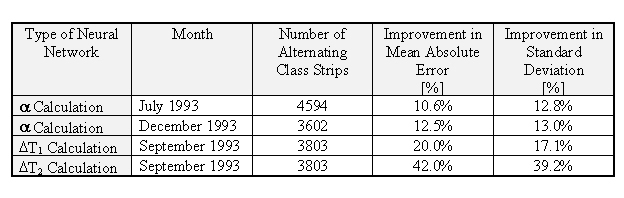
The use of this new approach of mathematical model, incorporating the use of neural networks, lead to an improvement in the mill performance, as can be seen in table IV. According to Siemens, improvements the calculation of hot rolling loads using neural networks are 20% more accurate than the values generated by classical methods. The improvement in strip temperature is about 35%. These first results were considered satisfactory; after all, since 1994 neural networks become a standard method used in every rolling mill automation systems delivered by Siemens [22]. However, work still continues on improvements in new versions of these hybrid models.
It is interesting to note that also Voest-Alpine developed its own hybrid automation system
for hot strip mill automation using mathematical modeling and neural networks, despite the
fact of its Linz Hot Strip Mill has a similar system delivered by Siemens [23]. However, there
are no published data available about the performance of Voest-Alpine system under industrial
conditions.
The approach of the Voest-Alpine for the calculation of hot strength of steel is somewhat different from Siemens. The practical use of the hybrid model showed that, for some kinds of steel, a specific value of a must be calculated for each rolling stand. So, it is being developed another neural network to identify such classes of steel that require calculation of several values of a [2]. One of the functions of this parameter is to emulate the microstructural refining that the rolling stock undergoes when it is deformed in successive rolling stands [15].
There is a work [13] describing with some detail a hybrid model mathematical model-neural network for the calculation of hot rolling load in a laboratory hot rolling mill. The calculation steps of this model are as follows:
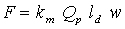 (1)
(1)where F is the roll separating force, km is the mean constrained flow stress in the roll bite for plane strain conditions, ld is the contact length, w is the rolling stock width and Qp is a geometric factor. While ld depends on the geometric configuration of the rolling mill and the stock being rolled, km can be calculated by the networks described in the items a) and b). Qp is defined by the equation
 (2)
(2)The original model of Alexander-Ford proposes the following formula for Q:
 (3)
(3)where hi and hf are the initial and final thickness of the rolled piece. The term Qp is strongly affected by the geometry of roll bite and interface conditions between the rolls and rolled piece. So, rolling parameters as lubricants, roughness of work roll and scale influence the value of this parameter, as this factor reflects the dynamic conditions of the mill. In order to improve the precision of this model, it was decided to calculate Qp using measured values of rolling load using the inverted model of Alexander-Ford. So, it was build a database containing all rolling data and the calculated values of Qp for 52 selected cases. The next step was to define a neural network for learn about the calculation of Qp from the information available on this database. It was verified that this parameter depends on the initial temperature and thickness, reduction and contact length; these variables constitute the input layer of the neural network. Two hidden layers with 12 neurons each were used, similar to the neural network applied for the hot strength calculation. The output layer has, naturally, only one neuron, the value of Qp. The training of this neural network required 80,000 iterations. The average error in the calculation of this parameter was equal to 0.022 %, with most of data within ± 2 % and maximum error within ± 6 %.
The calculation of roll load is as follows. First, the initial flow stress of the rolling
stock before rolling is calculated by the hot strength network. After that, the average
temperature in the roll bite is calculated by the temperature network. Then the exact value of
the average flow stress in the roll bite is re-calculated by the hot strength network. The
next step is the calculation of Qp by its corresponding network. Finally, the rolling load is
calculated by equation (1).
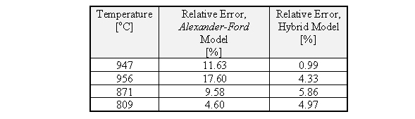
The precision of the global model was checked at one condition, a 15% reduction applied to a rolling stock with initial thickness equal to 9.2 mm. Table V shows the performance between the conventional Alexander-Ford model and the same model, but with Qp calculated by the neural network. It can be seen that it was got a impressive 75-90 % reduction in the relative errors at relatively high temperatures (950oC), whereas this reduction decreased to 39% at 870oC and, at 809oC, the performance of the conventional model was slightly better than the observed for the neural network.
- DETECTION OF “TURN-UP” DURING PLATE ROLLING
The turn-up, or excessive bowing upwards of rolled stock during plate rolling is a serious problem, as material being rolled can collide with the rolling stand or ancillary equipment’s, causing extensive damage. This problem was frequent at COSIPA’s plate mill, especially during the processing of Ni steels.
A previous work showed that alterations in the pass schedule could minimize the occurrence of turn-up, and led to the development of a statistical model for the calculation of an optimized pass schedule. It was showed then that there was a critical range of strain values to be avoided during plate rolling.
However, sometimes this statistical model calculated unfeasible values of roll gaps. In some cases the calculated values were excessively low, jeopardizing productivity; in other occasions, they were excessively high, well above the mill’s capacity of load, torque and power.
As soon the use of neural networks became available, it was a natural idea to use them in this application, as the statistical model was unsatisfactory [5]. After several trials, it was developed the following neural network:
The neurons number of the hidden layer of this neural network was calculated after the Hecht-Kolmogorov’s theorem, that was already mentioned. In fact, it was verified that this was the best configuration for maximizing the precision of this neural network.
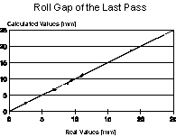
The developed neural network showed Pearson’s correlation coefficient r of 0.992 and standard error of estimate of approximately 3.0 mm. Figure 7 shows the dispersion plot of the real and calculated values. The most influencing variables, as indicated by the trained neural network, are turn-up index and initial roll gap distance, followed by rolling stock width, rolling load and work roll peripheral speed, considering a decreasing rank of importance.
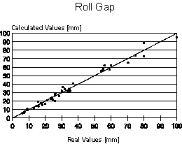
As can be seen in the graphic of figure 7, all calculated values are very near from the real
values. That is, the neural network did not generate non-sense values as the previous
developed regression polynomial equation.
The previous work about the turn-up occurrence in COSIPA’s plate mill had revealed that this defect was more frequent in a specific range of roll gap values, from 80 to 60 mm. This is confirmed by the trained neural networks, as the initial roll gap value is one of the most influencing variables of the model. Besides that, the standard error of estimate is admissible, as it is equal to only 7.5% of the minimum roll gap value. However, this is valid since the final thickness of plate is not located between 40 to 80 mm.
- LONGITUDINAL DISCARD CALCULATION WHEN USING PLANE VIEW CONTROL
Plate rolled from continuously cast slabs generally presents longitudinal extremities with “tongue” shape. This lowers the rectangularity index of the rolled stock, affecting its metallic yield, as irregular portions in the extremities of plate have to be cut. This characteristic can be attributed to the peculiar thickness profile of the continuously cast slabs. These slabs are slightly thicker in mid-width, resulting in a non-homogeneous mass distribution along the rolling stock, which affects the shape of its longitudinal extremities.
One solution proposed for this problem consists in the application of a special thickness profile in the rolling stock during the application of the last pass of the broadsizing step. After this special pass, the width of the rolling stock presents a thickness profile that basically consists of a “V”-shape notch or presents the shape of a “dog bone”. The development of this process in COSIPA led to a 0.7% increase in the metallic yield of the plate mill.
During the development of this process, it was developed a regression polynomial to correlate the “V”-shape notch depth and the total strain applied to the rolled stock after the broadsizing step with the length of the discarded portion of the final rolled stock, in order to have a better understanding of the process and check its optimization possibilities. This polynomial presented a Pearson correlation coefficient r of 0.903 and standard error of estimate of 132 mm.
Once more this appeared to be a good application for the neural networks technique, as it could be an opportunity to improve forecasting of the length of the discarded portion [5]. The best neural network designed to substitute the polynomial equation had the following configuration:
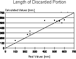
Although the neural network had showed better performance than the regression polynomial (the
standard error of estimation fell approximately 54%), errors observed in figure 8 still are
significant. Perhaps the cause of these relatively high errors stems from the use of the
discard length as an evaluation parameter of the metallic yield of the process. Really this
parameter is less representative than the weight or area of the discarded portion but, in
compensation, is an easier variable to be measured under industrial conditions.
- PASS SCHEDULE CALCULATION AIMING PLATE FLATNESS OPTIMIZATION
One of the most stringent quality parameters of plate is its flatness index. The traditional approach to flatness control during rolling consists to keep the rate crown variation : thickness variation within a restricted range, especially during the last three passes of the rolling schedule. This fact was also confirmed at COSIPA’s plate mill.
Mathematical models for the calculation of pass schedules are relatively easy to develop, but the use of neural networks is simpler. So, it was decided to use this new technique in this application too [5]. The three last passes of the rolling schedule were modeled regarding optimization of plate flatness; one neural network was attributed for each pass. The respective three neural networks showed the same configuration, as follows:
The flatness index used in this model varied in the range from 0 to 5: this index was greater as plate flatness worsened.
The performance of the neural network was very good. The Pearson’s correlation coefficient r corresponding to the last but two, penultimate and last pass were 0.998, 0.998 and 0.999, respectively; their standard error of estimate were 0.430, 0.394 and 0.140 mm, respectively. Figure 9 shows the dispersion plots of the real and calculated values for the three last passes of the rolling schedule.
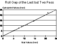
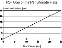
The most important variables in these neural networks were the aimed flatness index, the
original crown in the upper work roll and the rolling stock tonnage after the last change of
work rolls. Following to this group, there were parameters of intermediate importance like the
final plate width/thickness and temperature/load of the prior pass. Finally, variables like
prior pass flatness index/roll gap did not show great influence, but were vital to improve the
precision of the neural networks, making feasible its use under industrial conditions.
In fact, these neural networks identified during their “learning” step the most important variables related to flatness that are “traditionally” defined by the rolling theory: original crown of work rolls and rolling stock tonnage since change of work rolls. This last variable generally shows good correlation with thermal crown and wear of work rolls, factors that affect the resultant roll crown and, consequently, plate flatness. Work roll deflection promoted by rolling load was also considered, as this last variable was included in the input layer of the neural networks.
The last pass is the most important to define the final dimensions of plate, specially its thickness. The errors observed in the results calculated by the respective neural network varied from -0.26 to +0.17 mm, practically comprised within commercial plate thickness tolerance range. This results can be even improved, as a more precise data acquisition system becomes available, thus avoiding human errors during data collection and improving the precision of the measured parameters. Those facts undoubtedly will contribute to a better accuracy of these neural networks.
- PREDICTION OF PROCESS TEMPERATURES IN HOT STRIP MILLS
Neural networks were also used for the determination of the finishing temperature of rolling stock at the Hoogovens hot strip mill [24]. In this case, the input parameters were the same used in the traditional linear model incorporated to the automation system of the mill: re-predicted finishing temperature after the last stand; base finish rolling temperature, adapted from strip to strip; rolling speed of the last stand; strip thickness after the last finishing stand; calculated temperature at first finishing stand; and calculated temperature at first finishing stand. A feed-forward network, with one hidden layer, was used. The input layer had eight neurons, corresponding to the parameters already mentioned. Best results were got using seven neurons in the hidden layer. The output layer had only one neuron, corresponding to the finishing temperature.
The performance of the neural network model was 25% better than the previous linear statistical model. The relative standard deviation of the former model was about 6.0oC, while the neural network showed a value of 4.4oC. As neural networks are capable of handling different, non-linear dependencies in different areas of the input space, its prediction power generally is improved in comparison with linear models. In fact, a detailed analysis revealed that linear approximations seemed acceptable for most input parameters of the statistical linear model. However, relationship between the finishing temperature and some input parameters are clearly non-linear. This explains the better performance of the neural network model.
Strip cooling at the runout table of hot strip mills can also be modeled using neural networks. The first part of the hot strip mill runout table at the Port Talbot works of British Steel was modeled using neural networks [25]. Data used for training and testing of the neural network models consisted of 247 sets taken from three coils of C-Mn steel. They were all rolled in the same period, having identical target gauge, finishing temperature, interrupt temperature and coiling temperature.
Three feed-forward neural networks were tested. The input layer was the same for all these networks; it has eight neurons, corresponding to the finishing temperature, position of the coil segment in relation to the head end of the coil and water flow percentage of the first three top banks and the first three bottom banks. The output layer corresponded to the interrupt temperature, which is the strip temperature just after the first part of the runout table. Two of the proposed neural networks had only one hidden layer, with 20 and 4 neurons, respectively. The remaining network has two hidden layers, with 10 neurons each.
Surprisingly, the simpler neural network (one hidden layer with 4 neurons) showed best results, with an average error of 2.1oC and a maximum error of 14oC. This performance was far better than the standard model being used nowadays in the equipment, which showed an average error of 10.4oC and a maximum error of 25oC.
- PREDICTION OF AUSTENITIZING TEMPERATURES AND AUSTENITE TRANSFORMATION
A recently published work [26] showed the successful use of neural networks for the calculation of the Ac1 and Ac3 temperatures from the chemical composition of the alloy (in terms of contents of C, Si, Mn, S, P, Cu, Ni, Cr, Mo, Nb, V, Ti, Al, B, W, As, Sn, Zr, Co, N, O) and the heating rate used during the austenitizing treatment. The data set used for the training/testing steps of the neural network was gathered from TTT atlases; data from 788 alloys were compiled. The neural networks have only one hidden layer, which had four neurons for calculation of Ac1 and two neurons for Ac3. The lower number of neurons for the last neural network can be justified by the little influence from the starting temperature over Ac3. These models can estimate these transformation temperatures to an accuracy of about ±40oC (95% confidence limits). The analysis of the performance of these models showed that they extracted the correct metallurgical relationships between the heating rate/alloy content and these temperatures. The errors observed in the predictions can be largely attributed to the different starting microstructures in the samples used in the austenitization.
A previous work [27] used neural networks for the modeling of isothermal transformations diagrams (TTT diagrams) of hypoeutectoid heat treating steels with no microalloying elements. The input data for this network were the content of C, Mn (1.5% max.), Cr (3.0% max.), Ni (4.0% max.) and Mo (1.5% max.), plus the temperature (550oC being the lower limit for calculation). The boundary between ferrite and pearlite was not considered in this case.
The database considered for training of the neural networks derived from 52 alloys listed at the IRSID Atlas about transformation curves. Its training also considered that there is no transformation above the Ac3 temperature and the time to transformation was null if the austenitization temperature was lower than Ac3. Of course, also in this case neural networks were capable of determining the Ac1 and Ac3 from the chemical composition of the steel.
It was discovered that the best predicting neural network was also the most simple - one hidden layer with two neurons. Tests with similar alloys used in the training of the neural network revealed some tendency of greater errors in the range of low values of time, for both curves, transformation start and finish. However, the predictive capability of these neural networks was not quantitatively evaluated with detail. It was only verified that the influence of the data on the TTT diagram could only be effectively forecast by the neural network if the variation in the data exceeds ± 0.01% for C, Mn, Cr and Ni; ± 0.05 % for Mo and ± 5oC for the temperature. That is, considering two identical alloys, except by their Mo contents (0.30 and 0.34%, for instance), the comparison of both predictions carried out by the neural network could not correspond to the real effect that this alteration in the Mo content can produce.
Tests about the extrapolating power of these neural networks were carried out. It were observed errors of about 5 to 9% in the transformation start curve predictions, and up to 20% regarding the transformation finish curves.
Similar papers were published, describing neural networks for the calculation CCT diagrams [28] and martensite start temperature [29] from the chemical composition of steels.
The neural network developed in the first work calculates the start/end temperatures for the formation of ferrite, pearlite and bainite [28]. An important problem to be solved here is the conversion of the diagram into numerical format, which will be processed by the neural network. In this case, the intercepts of 23 fixed continuous cooling curves with the boundary lines indicating the time-temperature combination leading to a particular transformation product were determined. As relatively few data was available – only 89 vanadium steels, whose CCT diagrams were available from a single source – the training strategy was somewhat different from the usual, as it used cross-validation.
This complex problem was solved with a relatively simple feed-forward neural network, with three layers. The input layer had 13 neurons (austenitization temperature, C, Mn, Si, S, P, Cr, Ni, Mo, V, Cu, Al and N contents); the hidden layer had only 5 neurons and the output layer had 23 neurons, each one corresponding to a specific cooling curve. The performance of the neural network was relatively good for high and low cooling rates, presenting errors from 25 to 40oC. However, the observed error for intermediate cooling rates was greater, reaching eventually up to 100oC. The reason for this behavior can be explained by the greater complexity of the austenite transformation process that occurs under intermediate cooling rates and the ill-conditioned intersection angle between the cooling and the transformation curves along the intermediate cooling ranges of the CCT diagram. Besides that, the numerical conversion of the CCT diagram and the experimental errors inherent to its experimental determination also contributes to increase the error or the neural network model.
The effect of C and Mn over the Ar3 temperature (that is, ferrite transformation start), calculated by the neural network, yielded theoretically sound results: a decrease of 225oC per percent of C (since C content is less than 0.40%) and a decrease of 30oC per percent of Mn.
A bunch of empirical equations, developed through statistical multiple regression, was already available for the determination of the martensite start transformation [29]. In this case, it was proposed the calculation of martensite start temperature by a feed-forward neural network with 12 neurons in the input layer, representing the contents of C, Si, Mn, P, S, Cr, Mo, Ni, Al, Cu, N and V. Its hidden layer has six neurons. Of course, the output of the network is Ms,, the martensite start temperature.
Data used in the training and testing of this neural network was extracted from an atlas of continuous cooling transformation diagrams for vanadium steels. There was data available for 164 steel grades; 20 were selected for the validation of the network, while the remaining 144 were used for training.
The performance of this model in the prediction of the martensite start temperature was far better than the performance of the previously published regression equations. Its relative standard deviation was only 12oC, while this error varies between 34 and 61oC for the empirical equations. The neural network allowed also to verify the effect of some alloy elements over the value of Ms. This model clearly predicts a non-linear relationship between Ms and carbon concentration; this relationship varies with the base composition being considered. For its turn, manganese lead to a linear variation in Ms. It was also verified that the alterations in Ms promoted by Cr, Ni and V fall within experimental accuracy. The role of Mo was somewhat complex: for base alloys with 0.2% C it promotes an increase in Ms, while in base alloys with 0.4% the alterations in this parameter promoted by Mo fall within experimental accuracy.
Neural networks are being used also to the prediction of microstructure and final mechanical properties of hot rolled [30] or forged [31] steels. This kind of model is very complex, due to the extremely large number of parameters as inputs and many characteristic parameters as outputs. Some of these parameters do not directly affect microstructure, but indirectly through others, those have their own effect as well.
A proposed neural network used to predict microstructure and mechanical properties of hot rolled steels [30] use the following input variables: roll radius, entry thickness, exit thickness, rolling speed, entry temperature, exit temperature, times and cooling rates, the heat transfer coefficient, coefficient of friction, initial grain size and carbon content. The output of this model is the grain size at different locations of the cross section of the sample, roll force and roll torque. This network has one hidden layer with eleven neurons. Unfortunately, there is no information about the real performance of this model.
Another model was used to evaluate mechanical properties in forged parts [30]. The main objectives behind that project were support to alloy design and calculation of alloying additions during steelmaking. This neural network uses eleven elemental concentrations, one dimension variable and three process temperature variables as input parameters. The output parameters are the yield and tensile strengths. Unfortunately there are not more details about the real nature of the input data used in this model.
The neural network used in this example has one hidden layer with three neurons. There were 236 sets of industrial data available. Nine sets were eliminated as outliers. From the remaining 229 sets, 173 were used in the training and 56 in the test instance. The mean prediction error of this network in the test step was 5.5%, that is, about 50 MPa, slightly higher than the accuracy of the measured tensile and yield strengths, that was equal to 40 MPa. The use of 2, 4 or 5 neurons in the hidden layer lead to impairment of the precision got by the model. This model also allowed the verification of the effect of the input variables over the mechanical properties of the forged parts. It was found that the strongest nonlinear effects were due to boron and two of the temperature variables. The effect of titanium was also nonlinear, but not as strong as boron. On the other hand, there was practically no n onlinearity in the effect of chromium.
It is expected that this model can allow checking how much of a particular alloying element should be added to get the required properties. However, if the chemical composition is fixed, it is possible to alter strength by adjusting the process temperature variables.
- FEASIBILITY OF PRODUCTION OF A PARTICULAR STEEL SHAPE
Normally the decision about the feasibility of the production of a given steel grade or product is taken by an expert engineer, who intuitively evaluates the manufacturability difficulty grade of it. This ability is acquired through experience.
A model to systematize this technique in the specific case of shape steels, using a hybrid system, expert system and neural networks [31]. The function of the expert system is to select the neural network best fitted for the given case. The selected neural network simulates the judgement mechanism of the expert engineer, determining if the fabrication of a given product is feasible or not. Of course, this neural network must be previously trained with real examples to acquire the needed knowledge for this task.
An example of such neural network considers three variables: tensile strength lower limit, flange thickness and impact toughness guaranteed temperature. Their values are not directly input into the neural network. They are normalized according to a five level division. The values corresponding to each level are the data supplied to the neural network.
So, the input layer of the neural network has 15 neurons. Its hidden layer has 10 neurons. The output layer has five neurons, each one corresponding to a value of the manufacturing feasibility index. Only one neuron will react to a given set of data, signaling its corresponding manufacturing feasibility index. The first neuron of the output layer corresponds to the lowest value of the manufacturing feasibility index, that is, the worst condition of fabrication. For its turn, the last neuron corresponds to the maximum value of the manufacturing feasibility index, that is, the best condition of fabrication. The other neurons denote intermediate values of this manufacturing feasibility index.
- OTHER APPLICATIONS OF NEURAL NETWORKS IN HOT ROLLING PROCESS MODELING
The successful application of neural networks in the hot strip rolling load calculations motivated the development of other neural network models. Some of them are being used, while others still are being developed:
- CONCLUSION
Neural networks are not exactly a new modeling resource. Its fundamental principles were proposed in the 1940’s; the first hardware and software implementations were performed during the 1950’s and 1960’s; its development stalled in the late 1960’s due to hype and lack of theoretical background; it resurrected in the mid-1980’s, in function of further advancements on its theory and the wide availability of increasingly computer power at low costs. In the late eighties, both academic and commercial neural network software became available.
However, almost ten years after the resurgence of neural networks, its application in the field of hot rolling still is shy, in spite of the good results that were got. Few papers were published, although it is known that many steelworks tested the possibilities of this new technique. The majority of the cases described in the literature refer to laboratory experiments or industrial off-line models. In the few cases where neural networks were applied to real life hot rolling automation systems, they played a coadjuvant role, in the form of calculation of adaptive parameters to be used by the main conventional mathematical models.
This can be assigned to a lack of confidence on the performance of the neural networks. As its mathematical foundation still is not completely established, no one knows how their results are generated. So, even if its performance is good under practical conditions, fear about a sudden unexpected behavior still remains. Another aspect to be considered is the resistance to give up on former conventional models that took years and years to be refined.
Perhaps a more effective use of neural networks in the modeling of hot rolling processes is being considered more intensively in steelworks that still do not have hot rolling models developed. The possibility of quick and easy development of precise models from scratch using neural networks is tempting. However, the usual lack of instrumentation, data acquisition and computer facilities on these rolling mills still is hindering this possibility.
However, it must be noted that the industrial scale application of neural networks in hot rolling mills has effectively begun. The build-up of expertise and experience in the use of this new technique that will be collected along time undoubtedly will encourage further practical applications.
- REFERENCES

 |
Last Update: 05 October 2000 | |
| © Antonio Augusto Gorni |